axis([−2,2,−2,2]);
Mx = −2:0.5:2; My = −2:0.5:2;
[X1,X2] = meshgrid(Mx,My);
VX=X1+X2; VY=X1−X2;
quiver(Mx,My,VX,VY,’black’);2. Simulation
In this chapter, we will show how to perform a computer simulation of a nonlinear system described by its state equations:

This step is important in order to test the behavior of a system (controlled or not). Before presenting the simulation method, we will introduce the concept of vector fields. This concept will allow us to better understand the simulation method as well as certain behaviors that could appear in nonlinear systems. We will also give several concepts of graphics that are necessary for the graphical representation of our systems.
2.1. 벡터 필드의 개념
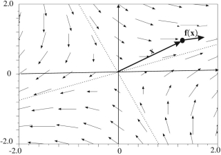
We will now present the concept of vector fields and show the manner in which they are useful in order to better understand the various behaviors of systems. We invite the readers to consult Khalil [KHA 02] for further details on this subject. A vector field is a continuous function f of Rn to Rn. When n = 2, a graphical representation of the function f can be imagined. For instance, the vector field associated with the linear function:

is illustrated in Figure 2.1. In order to obtain this figure, we have taken a set of vectors from the initial set, following a grid. Then, for each grid vector x, we have drawn its image vector f (x) by giving it the vector x as origin.
Figure 2.1. 선형 애플리케이션과 연관된 벡터 필드
The MATLAB code that allowed us to generate such a field is given below:
This program can also be found in the file field_syslin.m. We may recognize in this figure the characteristic spaces (dotted lines) of the linear application. We can also see that one eigenvalue is positive and another eigenvalue is negative. This can be verified by analyzing the matrix of our linear application given by:
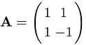
Its eigenvalues are images/ch2_Inline_3_11.gif and –images/ch2_Inline_3_11.gif and the associated eigenvectors are:
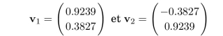
Let us note that the vector x represented in the figure is not an eigenvector, since x and f (x) are not collinear. However, all the vectors that belong to the characteristic subspaces (represented as dotted lines in the figure) are eigenvectors. Along the characteristic subspace associated with the negative eigenvalue, the field vectors tend to point toward 0, whereas these vectors point to infinity along the characteristic subspace associated with the positive eigenvalue.
For an autonomous system (in other words, one without input), the evolution is given by the equation images/ch2_Inline_3_8.gif. When f is a function of images/ch2_Inline_3_9.gif to images/ch2_Inline_3_10.gif, we can obtain a graphical representation of f by drawing the vector field associated with f. The graph will then allow us to better understand the behavior of our system.